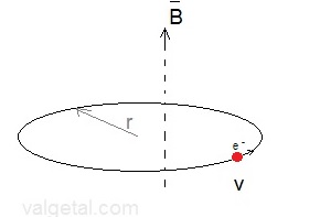
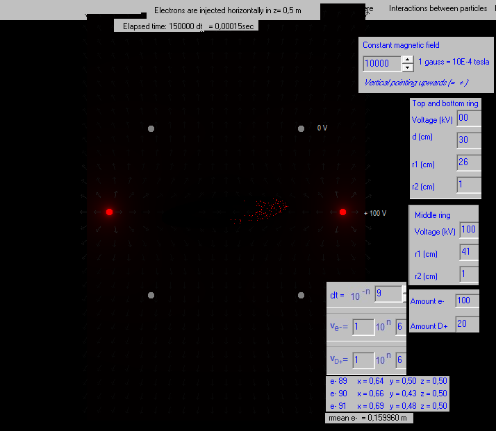
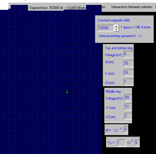
Let´s inject the electrons horizontally (in z=0,5 m)

Consider an electron moving in a magnetic field.

F = m.v² / r  -> B.q.v = m.v² / r 
F = Lorentz force on a moving charged particle in a magnetic field ( in newton)
v = speed of the electron (in m/s)
r = radius of the circular orbit of the electron (in meters)
m = 9.10 ×10⁻³¹ kg  (mass of the electron)

q = 1.6021×10⁻¹⁹ C (charge of the electron)

The electrons can be produced in an electron gun

They are accelerated by a voltage difference ΔV ->  q.ΔV = ½.m.v²

v = √(q. ΔV . 2. / m) = 5,930 . 10⁵ . √(ΔV)  m/s

Fig. 1

------------------

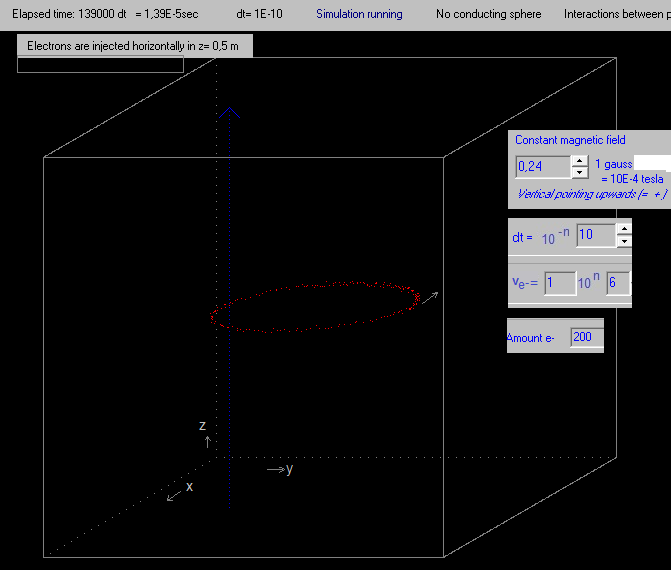
Fig. 2  exp. 14.1

B = 0,24 gauss
ve = 1,0.10⁶ m/s (speed of injected electrons)
no charged rings etc.
chcc:= 1; {an auxiliar variable}
electron[i].m:=chcc*me; {3E20 is the amount of D+ in the vacuum chamber if p=3E-2 torr};
electron[i].vx:=0 + (-0.5 + random)*ve/1000-vie; {vie = ve}
electron[i].vy:=0 + (-0.5 + random)*ve/1000;
electron[i].vz:=0 + (-0.5 + random)*ve/1000;
electron[i].q:=chcc*-qe;
electron[i].x:=0.50+ ( - 0.5 + random) /100; {so they do not start in exactly the same point};
electron[i].y:=0.5 + r1r - r2r - 0.05 + ( - 0.5 + random)/100;   { r1r  = inner radius up and bottom ring from vertical centre line, r2r = radius of cross section ring }
electron[i].z:=0.50+ ( - 0.5 + random) /100

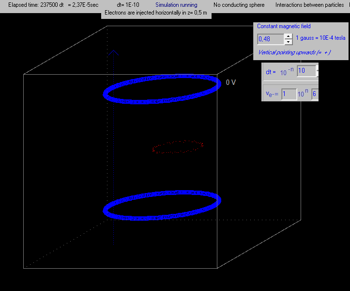
Remark: the speeds/velocities of the generated electrons are not exactly the same (see the code above -> Random function).
 

Fig. 3 exp. 14.2

All the same as in exp. 14.1, except the magnetic field B is twice as strong. As a result, the radius of the orbit of the
electrons is twice as small. (the sides of the cubes are 1 m).

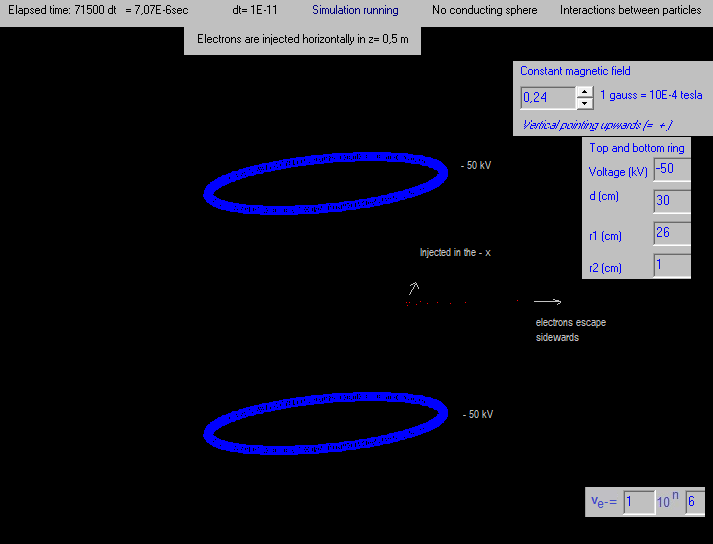
Fig. 4a exp. 14.3

If a negative voltage is applied to the blue rings, for example, -50 kV, then the electrons fly away sidewards, due to the
negative charge of the rings.The magnetic field is not strong enough to impede this. See fig. 4b.
 (d = distance between the rings, r1 = diameter rings, r2 = diameter cross section rings)

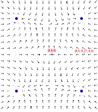
Fig. 4b exp. 14.3

The direction of the electric field is indicated, and two points (x,y,z),
for the experiment 14.3.

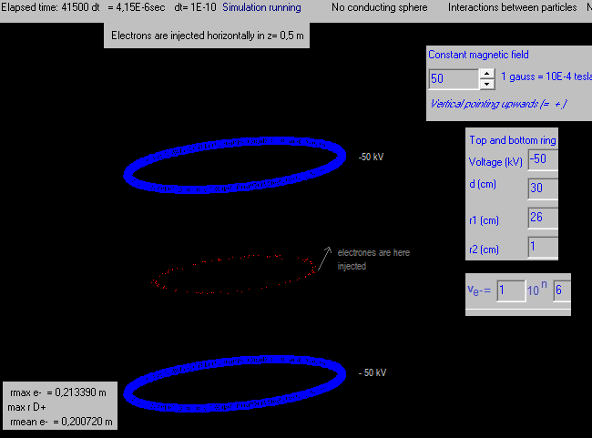
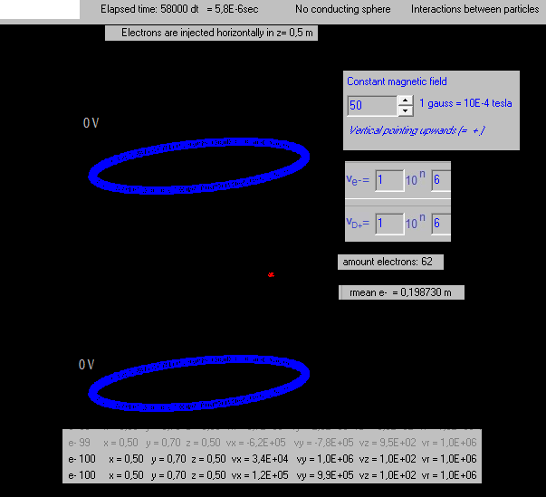
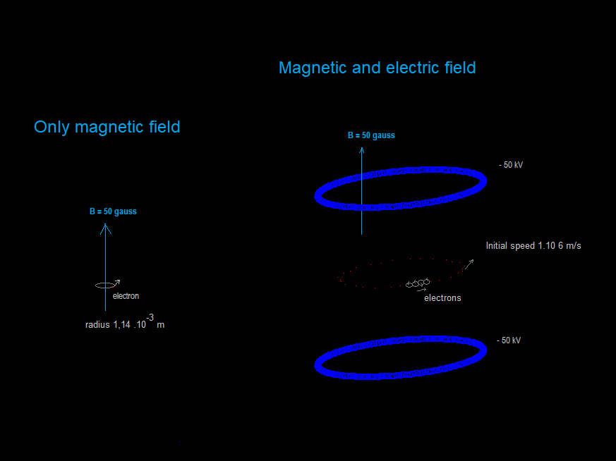
Fig. 5 exp. 14.4

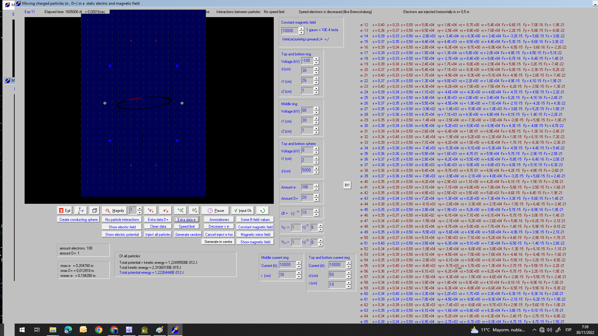
A vertical magnetic field of 50 gauss; the blue rings are charged with -50 kV.

The behaviour of the electrons is quite curious: they move in a big circle (not necessarily an exact circle) with a radius of about 0,20 m, but also in  small circles. The radius of the small circles (not necessarily exact circles) can hardly be seen. But the program has the possibiliy to magnify, and then it can be seen.

I suppose that the radius of the small circles is (about): r =  = m.v / ( B.q )  = 9.10 ×10⁻³¹ . (1,0.10⁶⁾ / (50.10^-4 . 1.6021×10⁻¹⁹  ) = 1,14 .10^-3 m

But why they move in the big circle?

Fig. 6 exp. 14.5

The big circle of the orbiting electrons is a tiny little bit smaller now. They still seem to move also in small circles.

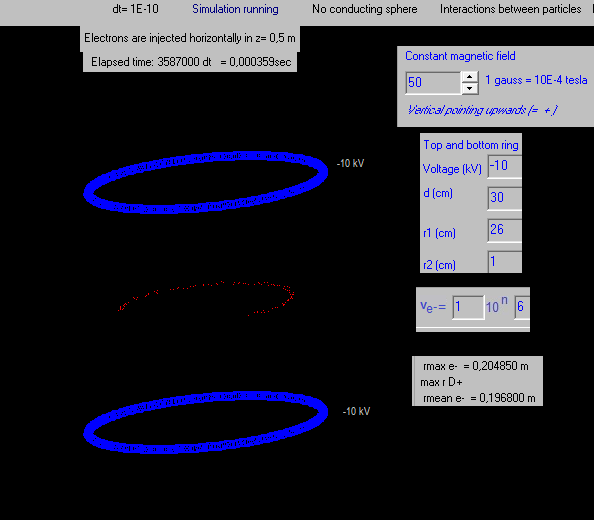
Fig. 7 exp. 14.6

The voltage of the blue rings is a bit smaller: - 5 kV.
Similar behaviour of the electrons.
mean e- is the mean radius of the electrons to the centre (0,0,0), not exactly the radius of the big circle

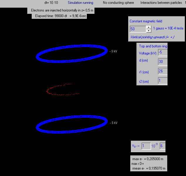
Exp. 14.6

All the same, only the voltage of the blue rings is now -1 kV.
The behaviour of the electrons is, more or less, the same.
The radius of the big circle is about 0,2 m

Fig. 7.b. Exp. 14.8

All the same, only the voltage of the blue rings is now 0 kV.

The electrons stay in the point where they are generated, it looks like they move
in small circles there with a small radius, possible the r = 1,12 .10^-3 m as calculated before.

Fig. 8.

Recording of various experiments in youtube

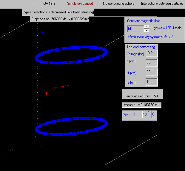
Remark: in exp. 14.9 till 14.14 dt=1E-9 is used, but for the electrons it is better to use dt=1E-10, because if the integration time dt is too large, it seems to be that the simulation program is "too slow" to calculate the fast moving light electrons.

Fig. 8. Exp. 14.9

All the same,  the voltage of the blue rings is -0.2 kV.

-----------

=> It seems to be that the more negative the voltage of the blue rings. the faster the electrones move
in the big circle (the speed tangential to the circle, or the meain speed of the swarm of electrons moving in the "big circle").
The radius of this big circle stays, more or less, the same.

Why?  This seems to be some curious interaction between the static electric field and the static magnetic field..

Let´s continue with different configurations.

--------------------------

Fig. 9. Exp. 14.10 (dt = 1E-9 s, but should be dt=1E-10 s)

Fig. 10. Exp. 14.11  (dt = 1E-9 s, but should be dt=1E-10 s)

The D+ ions do not stay well confined because the magnetic field strenght is only 300 gauss (0,03 T)

The electrons do circle/move in the big circle.

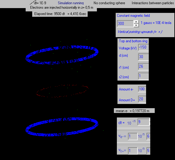
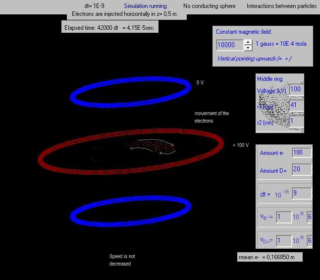
Fig. 11. Exp. 14.12 
(remark: the "swarm" movement seems to be caused because the integration time dt has been choosen too big: it should be dt= 1E-10 s and not 1E-9 s )

Under in the picture the swarm of electrons at three different times. They behave almost like a "swarm of starlings". (estorninos, spreeuwen, protters)
More or less a kind of circular motion around the vertical axis, but each electron also moves also in a kind of vibrating movement (or perhaps small circular movement).
By the way, the vertical distance of the electrons is all the time z=0,5 m (in the centre plane).

Video exp. 14.12   (at the right a 5x magnification )

Now the D+ ions stay better confined in this stronger magnetic field of 1 tesla.

I think it should be easier to inject the electrons from the side of the vacuum chamber, than vertically just above the bottom blue ring.

But because of bremsstrahlung the electrons will loose quite quickly their energy, and so their speed.
Let´s introduce this in the program and see what happens.

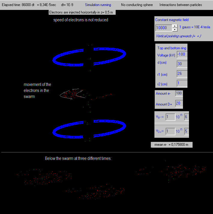
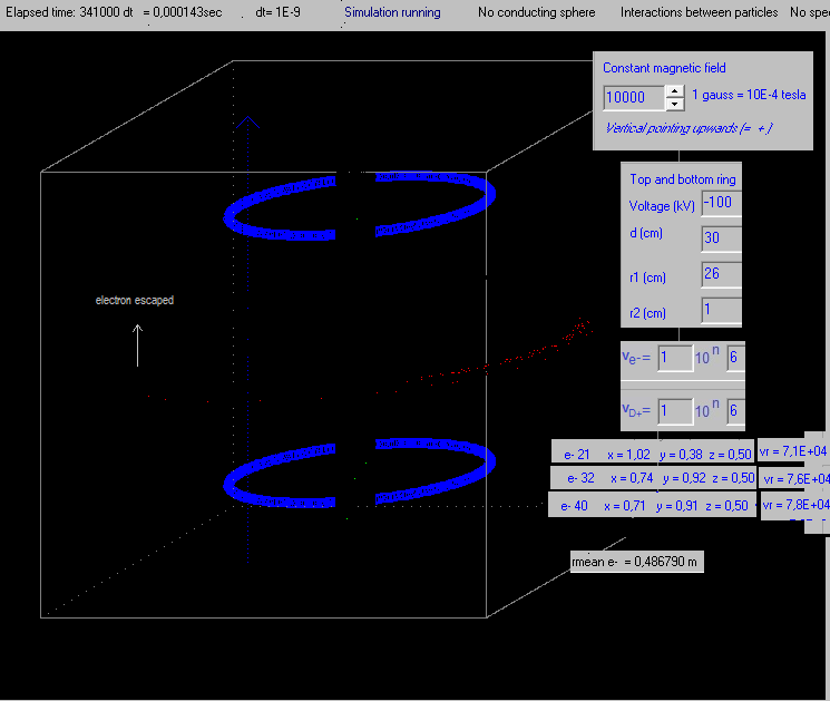
Fig. 12. Exp. 14.13  (dt = 1E-9 s, but should be dt=1E-10 s)

Exp 14.13 screenshot.png

if DecreaseSpeedElectrons=true then
begin
if t=1 then
begin
vx:=vx*0.999; vy:=vy*0.999; vz:=vz*0.999;
end;
end;

The speeds of the electrons descreases in time and they move then more to the outside. I saw one escaping.
The "swarm" is getting more narrow.

After 0,00018 s almost all electons escaped.

And when their speed is small, they are not longer well confined by the magnetic field,

It is a pitty that that they do not move to the centre, forming a kind of virtual electrode there :(

I did the experiment with dt=1E-10 s, decreasing the speed of the electrons, and they did also escape.

Fig. 13.

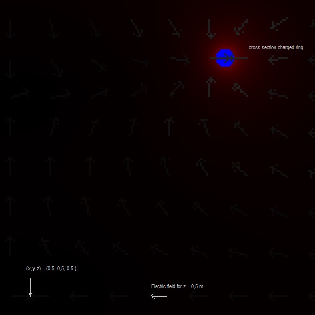
Here the direction of the electric field is shown, for the configuration of exp. 14.13
The electrons are generated in: x=0,5, y=0,5 (with a small random variation) and in
 y = 0.5 + r1r-r2r-0.05+ ( - 0.5 + random) /100
r1r = 0,26, r2r = 0.01 -> y = 0,70 m = 0,50 + 0,20 m ( with a small random variation)

In the centre x-y plane, the electric field is pointing towards the centre, so an electron will feel a electric force pointing outwards.
If there is no magnetic field, they escape sidewards. But with a magnetic field, the interaction of the magnetic and the electric
force on the electrons results in the simulation in the "swarm" movement as shown in the images.
 

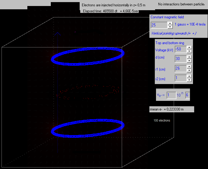
Fig. 14. Exp. 14.14 (dt = 1E-9 s, but should be dt=1E-10 s)

The electrons are injected in the same point (0,5, 0,7, 0,5 ), as in the former experiments.
electron[i].vx:=0 + (-0.5 + random)*ve/1000-vie;
electron[i].vy:=0 + (-0.5 + random)*ve/1000;
electron[i].vz:=0 + (-0.5 + random)*ve/1000+vie/2;

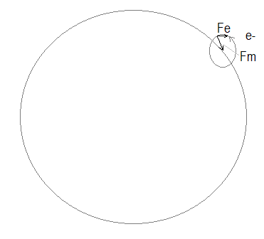
They have now also an initial speed vz upwards, but after being generated they start to move up an down (they do not escape vertically).
I suppose this is because when they are above or below the centre x-y plane, they are also above or below the positive charge red ring,
and hence they will feel a force back to the centre x-y plane.

Fig. 15. (x-y  centre plane)

Fe is the electric force exerted on the electron, pointing towards the positive ring.
Fm is the magnetic force exerted on the electron, pointing perpendicular to its velocity.

The interaction of these two forces should give as result the strange movement of the electrons as seen
in the simulation experiments.

Fig. 16. Exp. 14.14 (dt = 1E-9 s, but should be dt=1E-10 s)

The movement of the swarm of electrons is as shown above (a kind of caotic, vibrating movement, following more or less
the direction of the arrows, and the whole swarm moving in a "big" circle around the central vertical axis.

When the speed of the electrons is decreased in the program (like Brehmsstrahlung), they escape all, after some time.

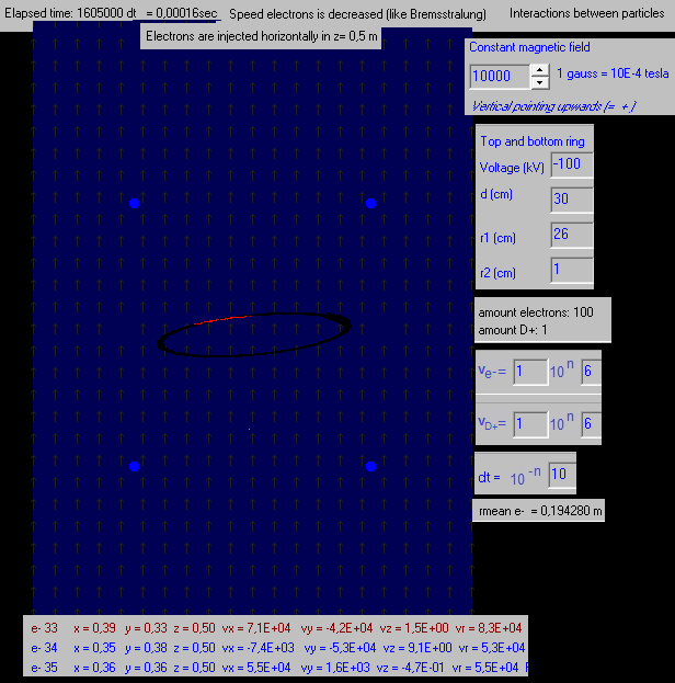
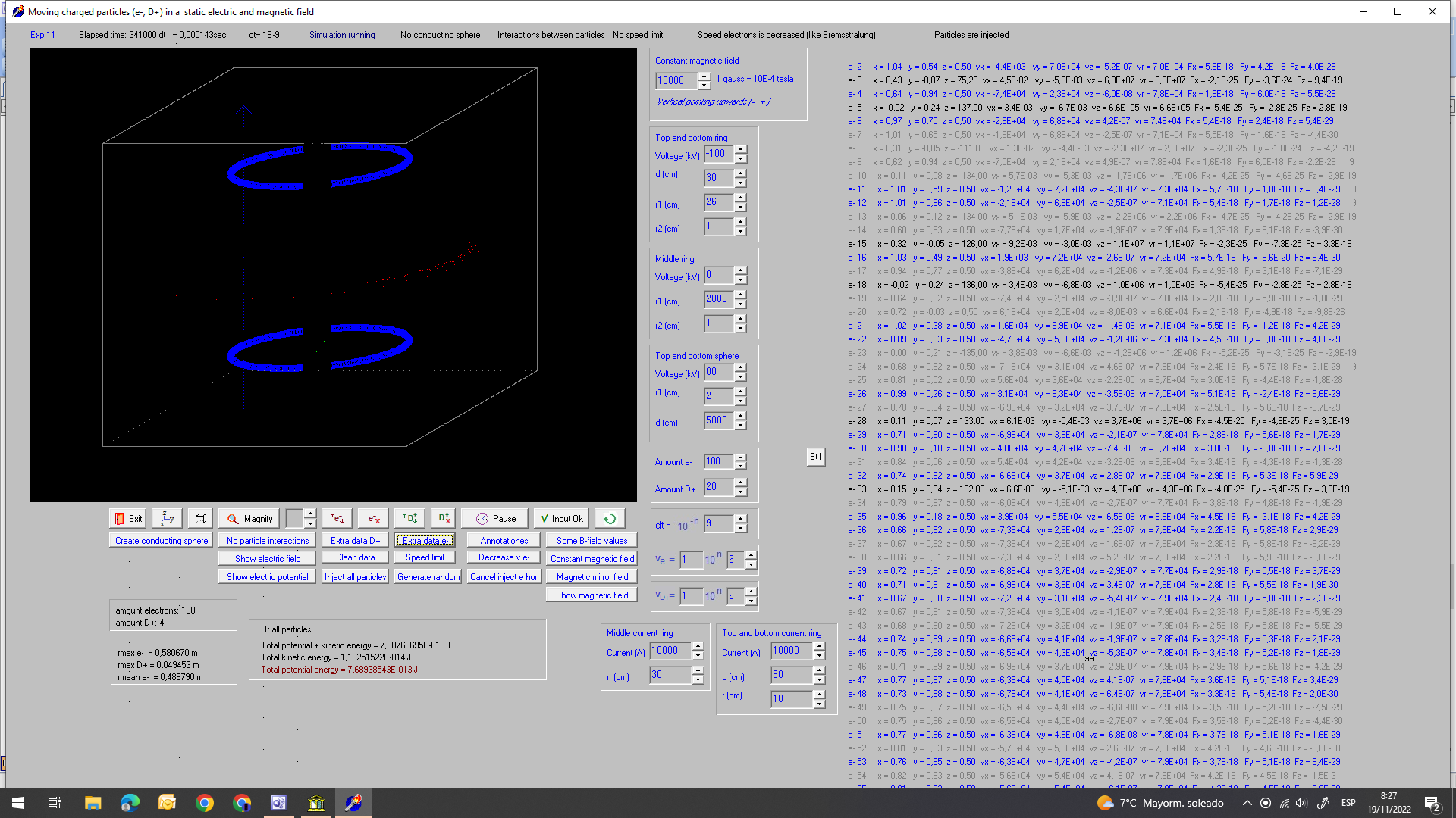
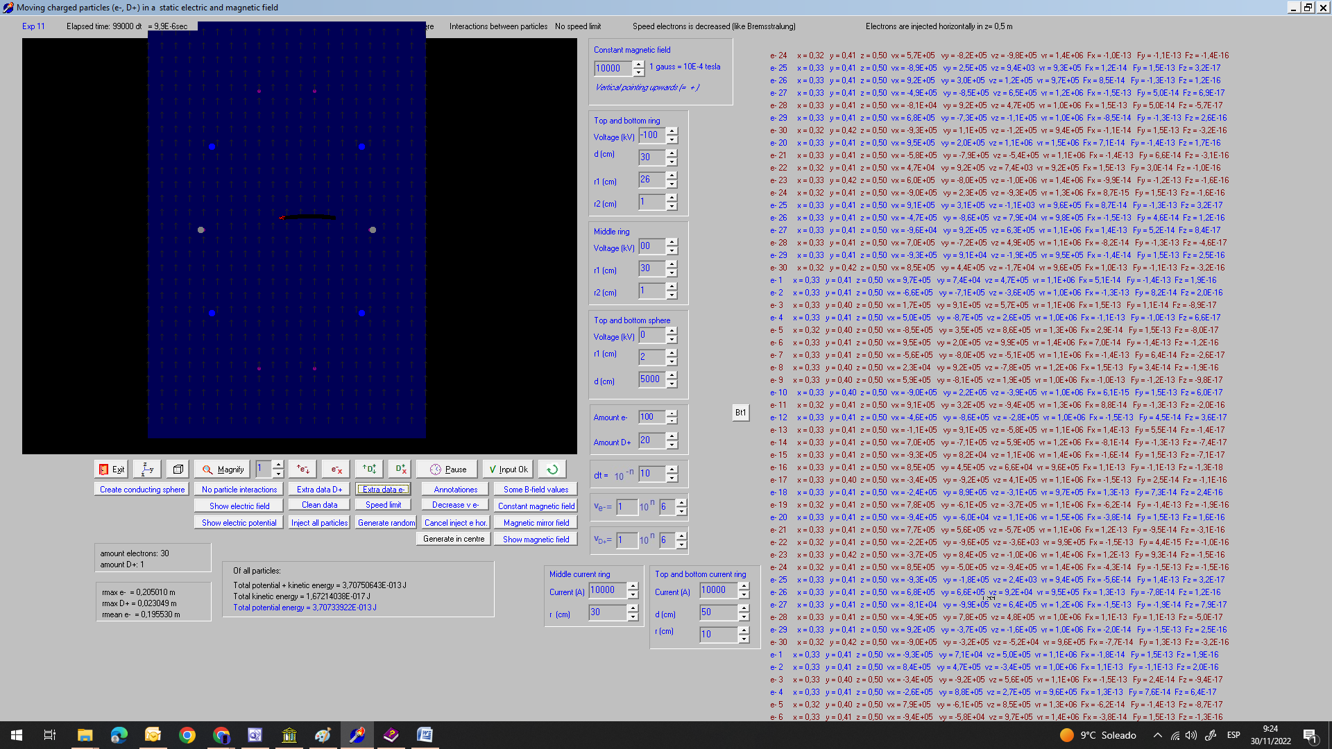
Fig. 17. Exp. 14.15

Exp. 14.15 screenshot.png

The same experiment as 14.13, only the integration time dt = 10^-10 s (instead of 10^-9 s)
The electrons move counter clockwise.

The speed of the electrons is reduced:
if (vx>1E1) and (vy>1E1) and (vz>1E1)
then
Begin
vx:=vx*0.90; vy:=vy*0.90; vz:=vz*0.90;

mean e- = mean radius electrons to the vertical z-axis. The radius fluctuates a bit in time, but stays more or less
the same (fig. 17 is the experiment after running one night, mean e- did almost not change).

The arrows show the direction of the magnetic field (is constant).

When the speed of the electrons is not reduced, they move more or less in the same way (also in this big circle), with mean e- = 0,1959 (changing in time a bit).

Exp. 14.15b  screenshot.png

Now with dt = 10^-10 s we do not see the "swarm of starlings movement",  as seen before, but they move still in the big circle. The speed with which the electrons move in the big circle depends of the negative potential of the rings: the higher the absolute value of this negative potential, the faster they move in the big circle.

Exp 14.15b.mp4 

Fig. 18. Exp. 14.16 Injecting D+ ions horizontally  without charged rings

De deuterium ions D+ are injected horizontally:
vid .= 1E5 m/s
hydrogen[i].vx:=0 +( - 0.5 + random)*ve/1000 - vid;
hydrogen[i].vy:=0 +( - 0.5 + random)*ve/1000; {random -> 0 <= X < 1 }
hydrogen[i].vz:=( - 0.5 + random)*ve/1000;
hydrogen[i].x:=0.5+( - 0.5 + random) /100 ;
hydrogen[i].y:= 0.5 + r1r-r2r-0.05+ ( - 0.5 + random) /100;
hydrogen[i].z:= 0.5+( - 0.5 + random) / 100;

The rings have potential 0 kV.

The D+ move in circles with r = m.v/(B.q) = 2.1,67E-27 . 1E5 /(1 . 1,6E-19) = 0,21 cm
Because they were given a small speed in the z-direction, they move "slowly" vertically.

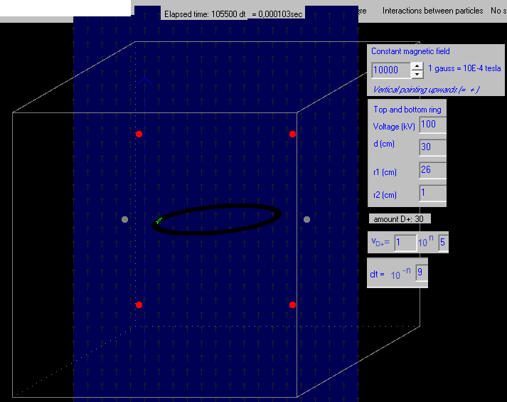
Fig. 19. Exp. 14.17  Injecting D+ ions horizontally  with charged rings at +100 kV

The same as exp. 14.16, only the two rings are now charged at +100 kV.

The D+ ions move clockwise in a big circle, simular as the electrons. (the electrons move counter clockwise).

With dt=10^-10 s they move also in the same big circle.
As far as I can observe, they do converge to the centre (the radius of the big circle seems to be, more or less, constant).

Fig. 19 Exp. 14.17 screenshot .png

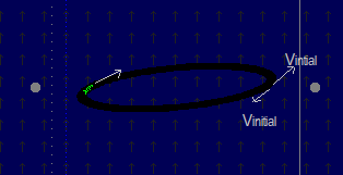
Also quite curious, it does not matter if you inject the D+  ions clockwise or counter clockwise, the always start moving clockwise in the big circle:

Fig.20.

(actually we did inject the particles at the right and the left,
but all started moving clockwise)

If InjectDhorizontally=true then

begin
hydrogen[i].vx:=0 +( - 0.5 + random)*ve/1000 - vid;
hydrogen[i].vy:=0 +( - 0.5 + random)*ve/1000; {random -> 0 <= X < 1 }
hydrogen[i].vz:=( - 0.5 + random)*ve/1000; {more or less with speed vid} {20}
hydrogen[i].x:=0.5+( - 0.5 + random) /100 {20}; {so they start not in exactly the same point}
hydrogen[i].y:= 0.5 + r1r-r2r-0.05+ ( - 0.5 + random) /100;
hydrogen[i].z:= 0.5+( - 0.5 + random) / 100;
hydrogen[i].exists:=true;
hydrogen[i].t:=2; {type=hydrogen}
hydrogen[i].i:=i;
form2.label54.caption:='amount D+: '+ IntToStr(i);

AmountH:=AmountH+1; {in initialisatie made zero, glob var in unit2}
i:=AmountH;
hydrogen[i].vx:=0 +( - 0.5 + random)*ve/1000 + vid   // -> + vid or - vid does not make any difference!
hydrogen[i].vy:=0 +( - 0.5 + random)*ve/1000; {random -> 0 <= X < 1 }
hydrogen[i].vz:=( - 0.5 + random)*ve/1000; {more or less with speed vid} {20}
hydrogen[i].x:=0.5+( - 0.5 + random) /100 {20}; {so they start not in exactly the same point}
hydrogen[i].y:= 0.5 - r1r+r2r+0.05+ ( - 0.5 + random) /100;
hydrogen[i].z:= 0.5+( - 0.5 + random) / 100;
hydrogen[i].exists:=true;
hydrogen[i].t:=2; {type=hydrogen}
hydrogen[i].i:=i;
form2.label54.caption:='amount D+: '+ IntToStr(i);
end else

------------------------------

Deflection of charged particles in a magnetic field in youtube

-----------------------------

Conclusion:

If we inject the electrons or the deuterium ions horizontally, they move, if the magnetic field is sufficiently strong and if the rings are charged, in a "big circle". The speed with which they move in this big circle depends of the potential of the rings: the higher the absolute potential of the rings, the faster the particles move in the ring.

This is quite a curious phenomenon, but I don´t know, for the moment, how to use this to improve the Sem Fusor design.

I also don´t know if I´ve made a new discovery, or if this is already known in the scientific world.

----------------------------

Via https://www.scienceforums.net/topic/128901-curious-behavior-of-electrons-in-a-static-electromagnetic-field/

I was told about:

https://groups.nscl.msu.edu/lebit/lebitfacility/penningtraps/index.html

October  2020 - February 2023    by  Rinze Joustra        www.valgetal.com